A Feasibility study using Monte Carlo Simulation

This work aimed to prepare a feasibility study for establishing a flexible packaging plant in Sofia, Bulgaria. The client was a well-known German industrial group. Whenever we need to make an informed decision about a particular investment, we rely on the help of a financial plan. In this plan, various variables are included as inputs that affect the final outcome and the likelihood of achieving a financial gain. In most cases, the financiers who prepare this plan rely on scenario analysis, with the options considered being good, bad and most likely scenarios. This approach relies on the managers' best guess about the value of the various variables included in the model. This deterministic approach does not include elements of randomness. You will get the same results whenever you run the model with the same set of initial input variables. On the other hand, a probabilistic model includes elements of randomness. Therefore, every time you run the model, you will get different results, even with the same initial conditions.

Monte Carlo simulation provides the decision-maker with a range of possible outcomes and their probabilities. It performs risk analysis by building models of possible results by substituting a base value of an input variable with a probability distribution. It then calculates results over thousands of iterations, each time using a different set of random values from the probability functions. The result is a distribution of possible outcome values for the variable of interest.
For further analysis, we have conducted a Monte Carlo simulation to show the range of possible outcomes in the model and tell how likely they are to occur. The method mathematically and objectively computes and tracks many different possible future scenarios, then tells the probabilities associated with each different one. This approach helps the investor to judge which risks to take and which ones to avoid, allowing for the best decision making under uncertainty.
This simulation aimed to find the probability distribution of the possible outcomes for IRR. The assumption is that several variables are stochastic, following their probability distributions. By simulating the results with 50'000 iterations, we have built a good estimate of the distribution of the outcomes. We prepared all calculations and charts using Decision Tools Suite – a risk and decision analysis toolkit from PALISADE.

What-If analysis

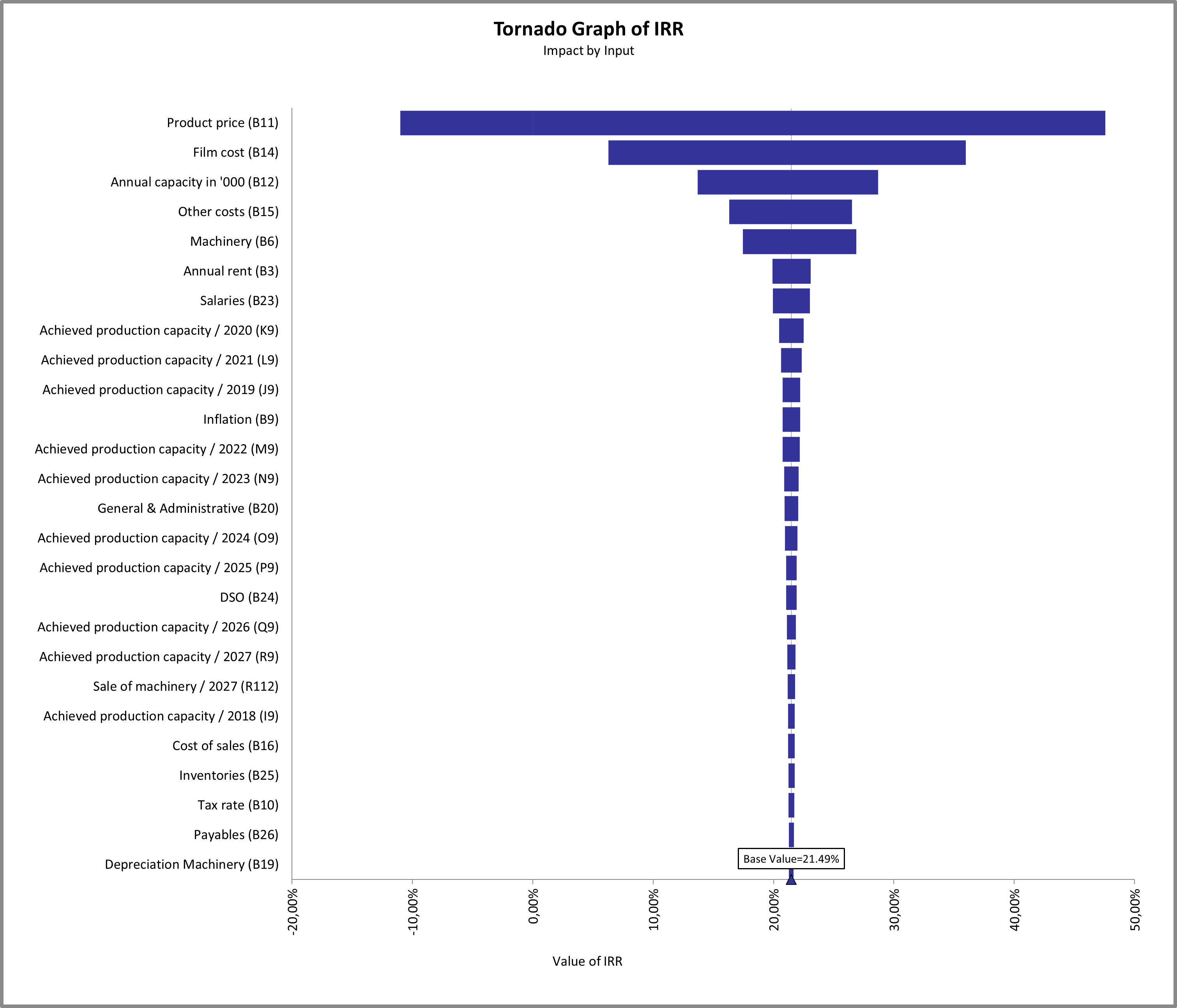
A first step in developing a risk model with many uncertain inputs is to understand which inputs have the most significant effect on the output, in our case, the IRR. We have used TopRank, an automated What-If analysis tool, to determine which model inputs have the biggest impact on IRR results. TopRank typically varies the value of each input, one input at a time, to see the effect of that input. According to their base values, we allowed the input values to vary in a What-If analysis from -20% to +20%. For example, these values are 3.28 and 4.92 for the variable "Product price". Below is the ranking of input variables according to their impact on IRR. In the table are all input variables, which change the output by more than 1%.

Picture 1: Tornado Graph

Monte Carlo Simulation

After identifying the most critical inputs, we can model these with @RISK probability functions, and the less essential inputs can be set at their base values.

We added the following uncertainties and assumptions:

• Product price: According to market data, the sale price of the end product varies with the foil price. The percentage increase in the price of foil is passed to the customer. We allowed the sale price to vary using PERT distribution with MIN, Most likely and MAX of -10%, base value (EUR 4.10) and +10%, respectively. This variability could come from contracting with the end customer and differences in the product mix.
• Film cost per kg: At the time of this report, we could not gather reliable data for BOPP historical prices. We assumed the cost of foil as fixed at the current level, meaning that the venture can
  pass any price increase to the customer. If historical BOPP prices are obtainable, the foil price can be modelled using time series analysis.
• Annual capacity in '000: This input is modelled with PERT distribution. The MIN value is 3'814 thousand kg (95% of the total capacity) due to the possibility of mechanical failure and other technical problems.
• Other costs per kg: These are allowed to vary using PERT distribution with MIN=-20%, Most likely=0,73 and MAX= +20%
• Machinery: We allowed the investment in machinery to vary using PERT distribution. MIN, M. likely and MAX are -20%, base value and +10%, respectively.
• Salaries: We allowed the annual salaries to vary using PERT distribution. MIN, M. likely and MAX are -10%, base value and +10%, respectively.
• Annual rent: The annual rent is modelled using PERT distribution. MIN, M. likely and MAX are -10%, base value and +10%, respectively.
• Annual inflation: The inflation rate is allowed to change between 0.5% and 3% using PERT distribution, with a most likely value of 1%.
• General & Administrative expenses: These vary between 1% and 3% from sales, with a most likely value of 2%.
• Sale of machinery: The selling price at the end of the period varies between EUR 3 mil and EUR 5 mil, with a most likely value of EUR 4 mil
• Cost of sales: These vary between 0.5% and 3% from sales, with a most likely value of 1%
• Days of sales outstanding (DSO): MIN, M. likely and MAX are 20 days, 30 days and 60 days, respectively
• The production capacity varies from 10% to 100%, depending on the availability of the production machines

After allowing for uncertainty, our analysis showed that the mean value of IRR drops from 21.49% to 20.44%, with a standard deviation of 3.25%. From all iterations, 63% of values for IRR are below 21.49%; what was the IRR value for the "no risk" model. Near 68% of the iterations are between two standard deviations.